🚀 Getting Started

Note

This example shows the interactive capabilities of Matplotlib backends, and this will not appear in the static documentation. Please run this code on your machine to see the interactivity.

This tutorial guides users through analyzing, visualizing, and generating synthetic birdsongs using the wavesongs Python package.

Google Colab Execution

If you are using Google Colabinstall the pacakge via pypi with the following code:

! git clone https://github.com/wavesongs/wavesongs
! pip install wavesongs
# enable hird party widgets (ipympl)
from google.colab import output
output.enable_custom_widget_manager()

In addition, you have to change the results and audio folder to:

audios = "/content/wavesongs/assets/audio"
results = "/content/wavesongs/assets/audio/results"

This is because in Google Colab all is downloaded at the contents folder.

Caution

If you encounter an error message, reset the kernel and run the above cell again. After that, everything should work successfully. Ensure that the audios and results variables are correctly set to the appropriate paths in your environment.

Libraries

Import the required classes and functions from wavesongs:

%matplotlib ipympl

from wavesongs.utils.paths import ProjDirs   # Manages project files
from wavesongs.objs.syllable import Syllable # Syllable ws objects
from wavesongs.objs.song import Song         # Song ws objects
from wavesongs import plot                   # Plotting utilities
from wavesongs.utils.tools import get_roi    # Data extraction tools

Important

The first line changes the Matplotlib backend to ipympl, enabling interactive plots. For more information about interactive plots, visit the official Matplotlib documentation on interactive figures. If you are using a Python or IPython terminal, omit this line.

Project Directory

To use objects like Syllable or Song, first define a project directory using a ProjDirs object. This object manages generated files such as images, audio files, and CSVs. The default project structure is:

📁 project_root
└── 📁 assets
    ├── 📁 audios
    |    ├── <audio sample files>
    |    └── <meta data>.csv
    └── 📁 results
        ├── 📁 audios
        ├── 📁 figures
        └── 📁 mg_params

audios = "./assets/audios"
results = "./assets/results"
proj_dirs = ProjDirs(audios=audios, results=results)

You can check the audio files found with the find_audios method

proj_dirs.find_audios()

['574179401 - Zonotrichia Capensis.wav',
 'XC388622 - Ocellated Tapaculo - Acropternis orthonyx.mp3',
 'XC553918.mp3',
 'XC11293.mp3',
 'XC542500.mp3',
 'XC842155.mp3',
 'XC380282.mp3']

Here are the audio samples that come with the package, the first two, and the samples downloaded from Xeno Canto in the 📥 Download Samples tutorial. These audios are stored in a folder with the name zonotrichia_capensis with their respective metadata in metadata.csv.

Song Object

Next, create a Song instance with the project directory and a file name. In this tutorial, we use the audio file 574179401 - Zonotrichia Capensis.wav located at assets/audio/ but you can use your own records or download samples from Xeno Canto.

Once the song is defined, compute its acoustic features. You can specify parameters such as the Fast Fourier Transform (FFT) window and fundamental frequency (FF) method.

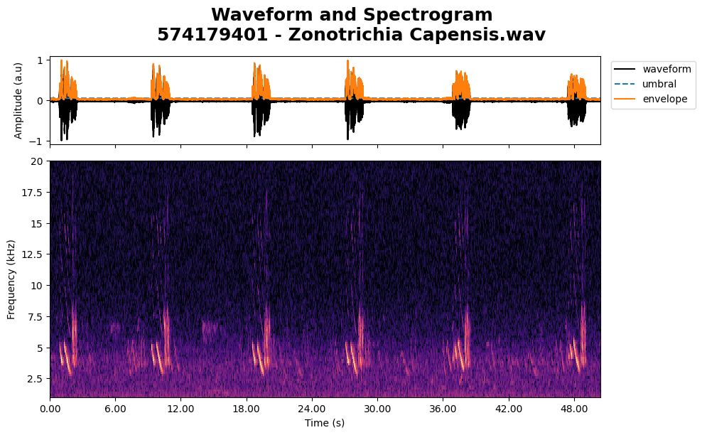
To display the spectrogram, use the plots module and the spectrogram_waveform function.

The name assigned to the song and syllables, “Copetón,” is the common name for Zonotrichia capensis in Colombia.

copeton_song = Song(proj_dirs, file_id="574179401")
copeton_song.acoustical_features(umbral_FF=1.4, NN=256)

# Display the song's spectrogram and waveform
plot.spectrogram_waveform(copeton_song, save=False)

copeton_song.play()

Tip

Long audio files can slow down plot response. A best practice is to define a region of interest (RoI), such as a complete birdsong.

Birdsong

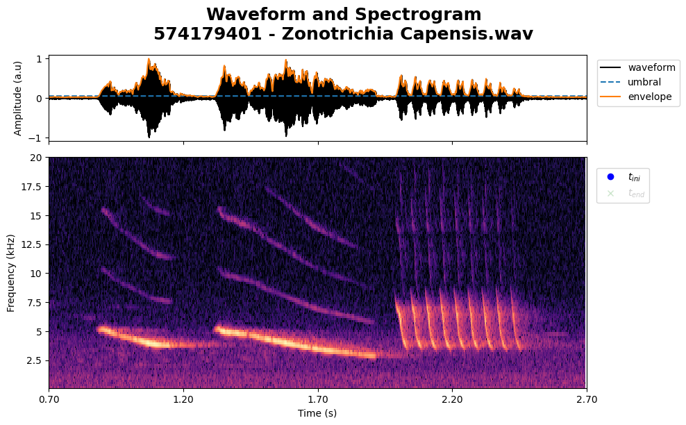
To select a specific time interval, set select_time=True and define the start and end of the RoI.

tlim_roi = (0.7, 2.7) # Time interval for the RoI

copeton_syllable = Song(proj_dirs, file_id="574179401", tlim=tlim_roi)
copeton_syllable.acoustical_features(umbral_FF=1.4, NN=256, ff_method="yin", flim=(1e2, 2e4))

klicker_times = plot.spectrogram_waveform(copeton_syllable, tlim=tlim_roi, select_time=True, save=False)

copeton_syllable.play()

This function returns an array of measurements, where each element is a vector containing time and frequency range values.

Warning

If no selection is made, an error will appear.

Note

The fundamental frequency is calculated using the YIN or PYIN algorithm. While the algorithm generally provides accurate results, the initial portion of the signal may not be computed as effectively.

data = get_roi(klicker_times)
tlim, flim = data[0] # index = 0: first pair
# Add the initial time from the syllable
t0 = tlim[0] + copeton_syllable.t0_bs
tend = tlim[1] + copeton_syllable.t0_bs
print(f"Region of Interest: (tini = {t0:.4f} s, tend = {tend:.4f} s)")

Region of Interest: (tini = 0.8781 s, tend = 1.3006 s)

Syllable

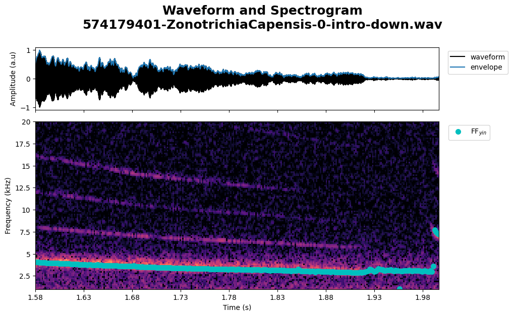
Define a syllable object within the selected RoI

# tlim = (0.8781, 1.3006) # For testing purpose
copeton_syllable_0 = Syllable(obj=copeton_syllable, tlim=tlim, type="intro-down", no_syllable="0")
copeton_syllable_0.acoustical_features(NN=256)

# Display the syllable's spectrogram and waveform
plot.spectrogram_waveform(copeton_syllable_0, ff_on=True, save=True)

Image save at ../../assets/results/figures/574179401-ZonotrichiaCapensis-0-intro-down

copeton_syllable_0.play()

# Write audio
copeton_syllable_0.write_audio()

Audio saved at ../../assets/results/audios/574179401-ZonotrichiaCapensis-syllable-0.wav.

Synthetic Syllable

To generate a synthetic syllable use the optimizer module, wavesongs.optimizer, which solves a minimization problem to find the optimal motor gesture coefficient such that generate the most similar syllable.

Optimal Coefficients

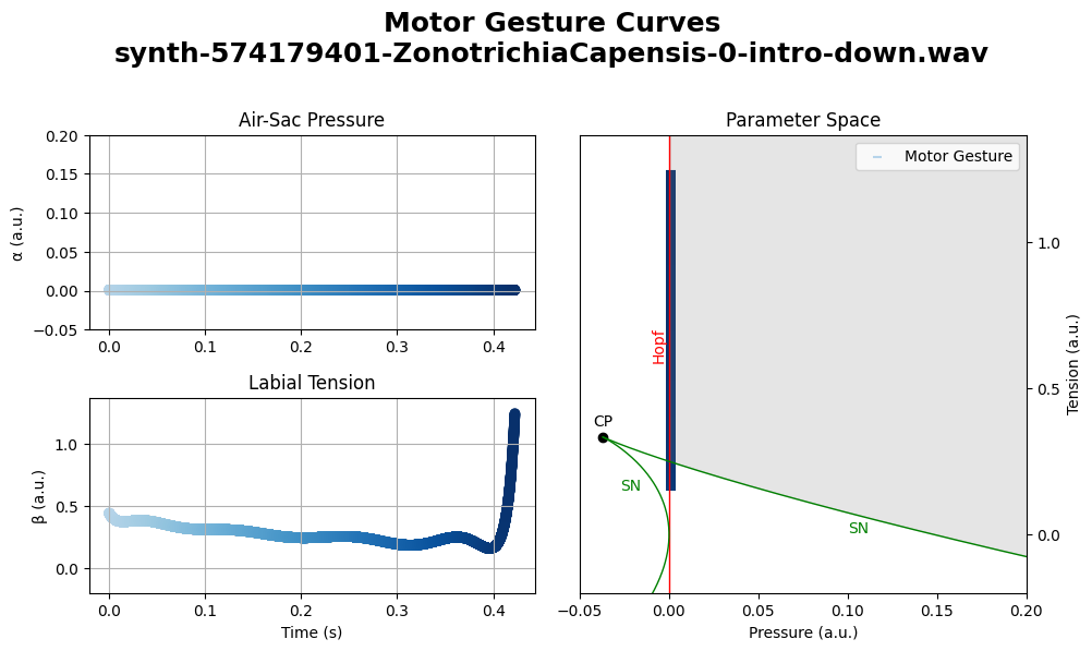
The birdsong model consists of four coefficients that define the labial tension (\(\beta\)) and air-sac pressure (\(\alpha\)): (\(a_0, b_0, b_1, b_2\)). Although both variables change over time, but we are just interested in the coefficients.

from wavesongs import optimizer

optimal_z = optimizer.optimal_params(syllable=copeton_syllable_0, Ns=10, full_output=True)
print(f"\nOptimal model values (alpha and beta coefficients):\n\t{optimal_z}")

Computing a0*...
Optimization terminated successfully.
         Current function value: 0.013981
         Iterations: 1
         Function evaluations: 2
	 Optimal values: a_0=0.0010, t=0.76 min

Computing b0*, b1*, and b2*...
Optimization terminated successfully.
         Current function value: 0.003349
         Iterations: 37
         Function evaluations: 75
	 Optimal values: b_0=-0.1973, b_2=1.2033, t=20.21 min
Optimization terminated successfully.
         Current function value: 0.003350
         Iterations: 13
         Function evaluations: 27
	 Optimal values: b_1=0.9992, t=6.27 min

Time of execution: 27.24 min

Optimal model values (alpha and beta coefficients):
	{'a0': 0.00105, 'b0': -0.19726, 'b1': 0.99924, 'b2': 1.20333}

Solution

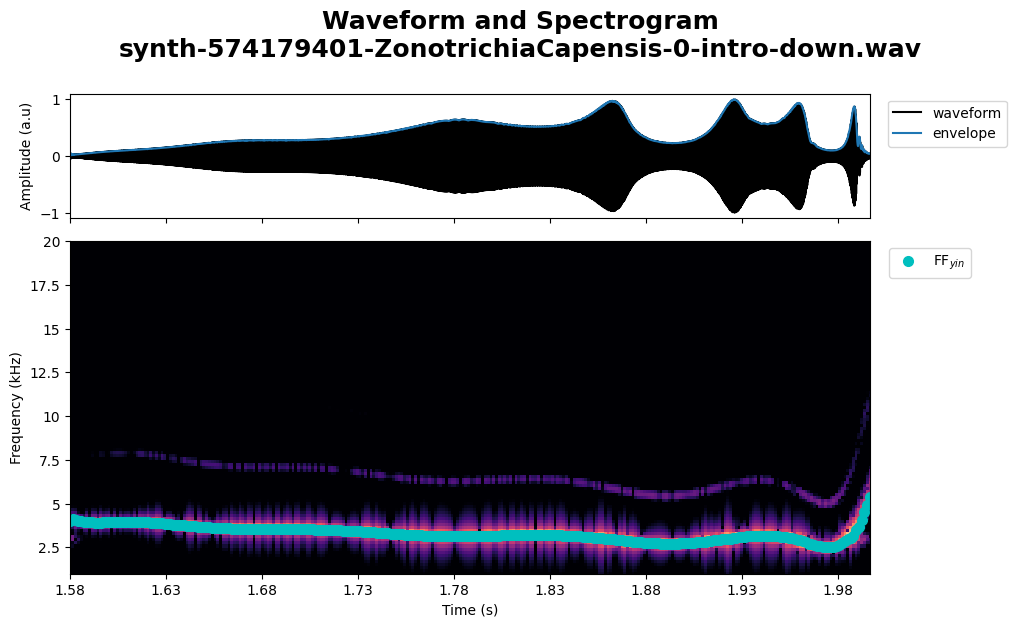
Now, generate and visualize the synthetic syllable using the computed optimal coefficients, optimal_z.

# optimal_z = {'a0': 0.00105, 'b0': -0.19726, 'b1': 0.99924, 'b2': 1.20333} # Testing purpose
synth_copeton_syllable_0 = copeton_syllable_0.solve(z=optimal_z, method="best")
plot.spectrogram_waveform(synth_copeton_syllable_0, ff_on=True, save=True)

Image save at ../../assets/results/figures/synth-574179401-ZonotrichiaCapensis-0-intro-down

synth_copeton_syllable_0.play()

# Write synthetic sample
synth_copeton_syllable_0.write_audio()

Audio saved at ../../assets/results/audios/synth-574179401-ZonotrichiaCapensis-synth-syllable-0.wav.

In the solve() method, there are two approaches available for generating synthetic songs:

1. best Method: The labial tension is calculated using the formula:

   \[ \beta(t) = b_0 + b_1 \cdot \tilde{FF} + b_2 \cdot \tilde{FF}^2 \]

   where \(\tilde{FF}\) represents the fundamental frequency normalized by \(10^4\) Hz.

2. fast Method: The labial tension is computed as:

   \[ \beta(t) = b_0 + b_1 \cdot t + b_2 \cdot t^2 \]

   where \(t\) denotes time.

Additionally, you can export and import the entire Syllable object for further use or analysis.

Saving Curves

Export

Exporting syllable parameters

synth_copeton_syllable_0.export_mg(export_curves=True)

Curves arrays saved at ../../assets/results/mg_params/synth-574179401-ZonotrichiaCapensis-0-curves.csv
Motor gesture parameters saved at ../../assets/results/mg_params/574179401-ZonotrichiaCapensis-0-mg.csv.

Import

Importing parameters from csv file

proj_dirs = ProjDirs(audios="../../assets/audio", results="../../assets/results")
imported_synth_copeton_syllable_0 = proj_dirs.import_mg("574179401", no_syllable=0)
plot.spectrogram_waveform(imported_synth_copeton_syllable_0, ff_on=True)

Image save at ../../assets/results/figures/synth-574179401-ZonotrichiaCapensis-0-intro-down

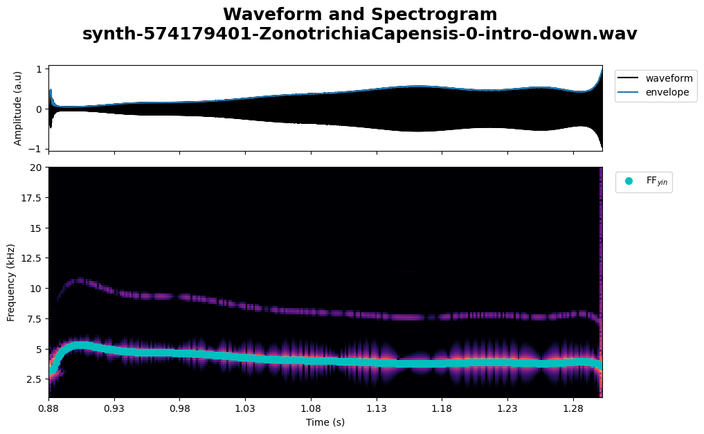
This process generates a CSV file containing all the parameters of the Syllable. The file name ends with "mg". If the best method is selected, an additional file will be created during export, ending with "curve". This file includes the curve arrays for time (\(t\)), air-sac pressure (\(\alpha(t)\)), and labial tension (\(\beta(t)\)). By default, both files are stored in the directory assets/results/mg_params/.

imported_synth_copeton_syllable_0.play()

Plots

Comparing Samples

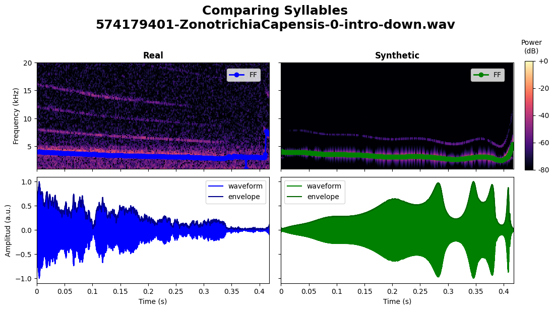
plot.syllables(copeton_syllable_0, synth_copeton_syllable_0, ff_on=True)

Image save at 574179401-ZonotrichiaCapensis-0-intro-down-SoundAndSpectros.png

Motor Gesture

plot.alpha_beta(synth_copeton_syllable_0)

Image save at synth-574179401-ZonotrichiaCapensis-0-intro-down-mg_params.png

Physical Variables

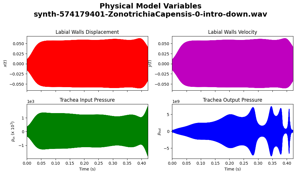
plot.phsyical_variables(synth_copeton_syllable_0)

Image save at synth-574179401-ZonotrichiaCapensis-0-intro-down-PhysicalVariables.png

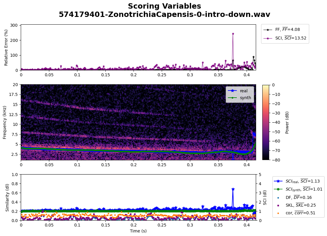
Score Variables

plot.scores(copeton_syllable_0, synth_copeton_syllable_0, save=True)

Image save at 574179401-ZonotrichiaCapensis-0-intro-down-ScoringVariables.png

---

This tutorial introduced WaveSongs for bioacoustic analysis, covering setup, song processing, spectrogram visualization, and synthetic syllable generation. By following these steps, you can analyze bird vocalizations and optimize synthetic models for research or educational purposes.

Happy coding! 🎵🔬